Interpreting a leaf identification model with LIME

This notebook demonstrates the use of DIANNA with the LIME method on the leafsnap30 image dataset. A pre-trained neural network classifier is used, which identifies the species of leaf based on an image of it.

LIME (Local Interpretable Model-agnostic Explanations) is an explainable-AI method that aims to create an interpretable model that locally represents the classifier. For more details see the LIME paper.

NOTE: This tutorial is still work-in-progress, the final results need to be improved by tweaking the LIME parameters

Colab Setup

running_in_colab = 'google.colab' in str(get_ipython())
if running_in_colab:
  # install dianna
  !python3 -m pip install dianna[notebooks]

  # download data used in this demo
  import os
  base_url = 'https://raw.githubusercontent.com/dianna-ai/dianna/main/dianna/'
  paths_to_download = ['./data/leafsnap_example_acer_rubrum.jpg', './labels/leafsnap_classes.csv', './models/leafsnap_model.onnx']
  for path in paths_to_download:
      !wget {base_url + path} -P {os.path.dirname(path)}

0 - Imports and paths

from PIL import Image
import matplotlib.pyplot as plt
import numpy as np
from pathlib import Path

import dianna
from dianna import visualization

true_species = 'acer_rubrum'
image_path = Path('..','..','..','dianna','data', f'leafsnap_example_{true_species}.jpg')
model_path = Path('..','..','..','dianna','models', 'leafsnap_model.onnx')
model_classes_path = Path('..','..','..','dianna','labels' ,'leafsnap_classes.csv')

1 - Loading the data

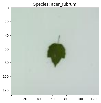
Two files are loaded here: 1. A file containg the numerical index that belongs to each class (=species of leaf). This is used so we know which output of the neural network corresponds to the class we want to run LIME on. 2. An image of a leaf, belonging to the Acer Rubrum species.

DIANNA requires input in numpy format, so the .jpg image is loaded and converted into a numpy array. The pixel values are then converted to the 0-1 range, which the classifier requires. Finally, DIANNA requires the presence of a batch axis, and it needs to know where the batch and colour channel axes are located in the input data.

# load the model class definitions
class_to_idx = dict(np.genfromtxt(model_classes_path, dtype=None, encoding=None, delimiter=','))
true_species = 'acer_rubrum'
true_species_index = class_to_idx[true_species]

# load and plot the example image
img = np.array(Image.open(Path('..','..','..','dianna','data', f'leafsnap_example_{true_species}.jpg')))

plt.imshow(img)
plt.title(f'Species: {true_species}');

# the model expects float32 values in the 0-1 range for each pixel, with the colour channels as first axis
# the .jpg file has 0-255 ints with the channel axis last so it needs to be changed
input_data = img.transpose(2, 0, 1).astype(np.float32) / 255.

# define axis labels. Required is the channels axis
# in this example image, the channels axis is the first axis
axis_labels = {0: 'channels'}

2 - Applying LIME with DIANNA

The simplest way to run DIANNA on image data is with dianna.explain_image. The arguments are: * The path to the model in ONNX format * The image we want to explain * The name of the explainable-AI method we want to use, here LIME * The location of the batch and colour channel axes in the data * The numerical indices of the classes we want an explanation for

# An explanation is returned for each label, but we ask for just one label so the output is a list of length one.
explanation_heatmap = dianna.explain_image(model_path, input_data, 'LIME', axis_labels=axis_labels, labels=[true_species_index])[0]

3 - Visualization

DIANNA includes a visualization package, capable of overlaying the explanation heatmap on the original input image.

In this visualization, important superpixels are red, while less important superpixels are blue.

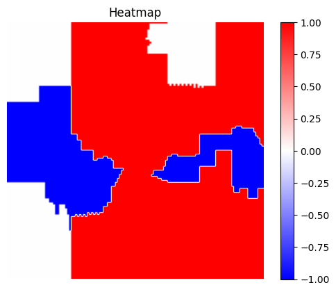
visualization.plot_image(explanation_heatmap, heatmap_cmap='bwr')
plt.title('Heatmap')
plt.axis('off')

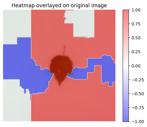
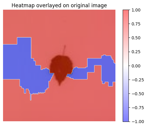
visualization.plot_image(explanation_heatmap, original_data=img, heatmap_cmap='bwr')
plt.title('Heatmap overlayed on original image')
plt.axis('off')

plt.show()

The output heatmap is not very informative, there are only a few large blocks without much detail.

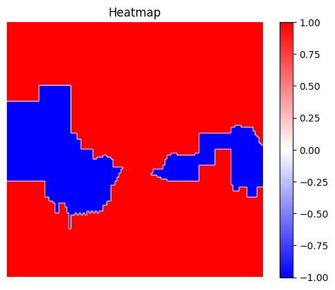
We can run LIME again with some customized values for some of the options. These options can be given to dianna.explain_image and will automatically be used by LIME.

We will change two things: * Increase the number of features from the default 10 to 30 * Change the colour of superpixels that are turned “off” by LIME to white (Default = average of surrounding superpixels)

explanation_heatmap_customized = dianna.explain_image(model_path, input_data, 'LIME', axis_labels=axis_labels, labels=[true_species_index],
                                                    num_features=30, num_samples=1000)[0]

visualization.plot_image(explanation_heatmap_customized, heatmap_cmap='bwr')
plt.title('Heatmap')
plt.axis('off')

visualization.plot_image(explanation_heatmap_customized, original_data=img, heatmap_cmap='bwr')
plt.title('Heatmap overlayed on original image')
plt.axis('off')

plt.show()