Interpreting a weather classification model with LIME

This notebook demonstrates the use of DIANNA with the LIME timeseries method on the weather dataset.

LIME (Local Interpretable Model-agnostic Explanations) is an explainable-AI method that aims to create an interpretable model that locally represents the classifier. For more details see the LIME paper.

NOTE: This tutorial is still work-in-progress, the final results need to be improved by tweaking the LIME parameters

Colab Setup

running_in_colab = 'google.colab' in str(get_ipython())
if running_in_colab:
  # install dianna
  !python3 -m pip install dianna[notebooks]

  # download data used in this demo
  import os
  base_url = 'https://raw.githubusercontent.com/dianna-ai/dianna/main/dianna/'
  paths_to_download = ['./models/season_prediction_model_temp_max_binary.onnx']
  for path in paths_to_download:
      !wget {base_url + path} -P {os.path.dirname(path)}

0 - Libraries

import os
import pandas as pd
import numpy as np
from dianna import visualization
from matplotlib import pyplot as plt
from sklearn.model_selection import train_test_split
import onnx
import onnxruntime as ort
import dianna

np.random.seed(0)

1 - Create a mini dataset with extremes for verification

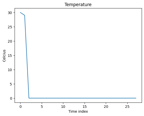
To demonstrate the skill of RISE for timeseries model explanation, we “make up” a weather dataset (timeseries) with extrem hot days and cold days.

# make up a weather dataset with extrems
cold_with_2_hot_days = np.expand_dims(np.array([30, 29] + list(np.zeros(26))) , axis=1)
data_extreme = cold_with_2_hot_days
fig = plt.figure()
plt.plot(data_extreme)
plt.xlabel("Time index")
plt.ylabel("Celcius")
plt.title("Temperature")
plt.show()

2 - Define an “expert” model to verify RISE for timeseries

We can define an ‘expert’ model to test RISE. This expert model decides it’s summer if the mean temp is above the threshold, and winter in other cases.

# We define a threshold for the model to make decisions
# The label is ["summer", "winter"]
threshold = 14

def run_expert_model(data):
    is_summer = np.mean(np.mean(data, axis=1), axis=1) > threshold
    number_of_classes = 2
    number_of_instances = data.shape[0]
    result = np.zeros((number_of_instances ,number_of_classes))
    result[is_summer] = [1.0, 0.0]
    result[~is_summer] = [0.0, 1.0]
    return result

3 - Compute and visualize the relevance scores

In this section we compute the relevance scores for each segment of timeseries using LIME and visualize them on the original timeseries.

# we use the threshold to mask the data
def input_train_mean(_data):
    return threshold

exp = dianna.explain_timeseries(run_expert_model, input_timeseries=data_extreme,
                                method='lime', labels=[0,1], class_names=["summer", "winter"],
                                num_features=len(data_extreme), num_samples=10000,
                                num_slices=len(data_extreme), distance_method='euclidean',
                                mask_type=input_train_mean)

Explaining: 100%|████████████████████████████████████████████████████████| 10000/10000 [00:00<00:00, 34484.38it/s]

Now we can visualize the relevance scores on top of the displayed timeseries using the visualization tool in dianna.

# Normalize the explanation scores for the purpose of visualization
def normalize(data):
    """Squash all values into [-1,1] range."""
    zero_to_one = (data - np.min(data)) / (np.max(data) - np.min(data))
    return 2*zero_to_one -1

heatmap_channel = normalize(exp[0])
segments = []
for i in range(len(heatmap_channel) - 1):
    segments.append({
        'index': i,
        'start': i - 0.5,
        'stop': i + 0.5,
        'weight': heatmap_channel[i]})
fig, _ = visualization.plot_timeseries(range(len(heatmap_channel)), data_extreme,
                              segments, x_label="Time index", y_label="Temperature")

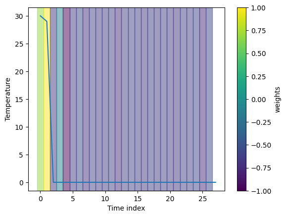
Here we plot the explanation for the classification of summer. The results are consistent with our expectation as it marks all hot days in the timeseries.

Now let’s try out LIME with a weather prediction dataset from real life. Here is the doi to this dataset: 10.5281/zenodo.4770936

4 - Loading the weather prediction dataset

Downloading the weather prediction dataset from zenodo.

# Load weather dataset
fname = "weather_prediction_dataset.csv"
if os.path.isfile(fname):
    data = pd.read_csv(fname)
else:
    data = pd.read_csv(f"https://zenodo.org/record/7525955/files/{fname}?download=1")
data.describe()

	DATE	MONTH	BASEL_cloud_cover	BASEL_humidity	BASEL_pressure	BASEL_global_radiation	BASEL_precipitation	BASEL_sunshine	BASEL_temp_mean	BASEL_temp_min	...	STOCKHOLM_temp_min	STOCKHOLM_temp_max	TOURS_wind_speed	TOURS_humidity	TOURS_pressure	TOURS_global_radiation	TOURS_precipitation	TOURS_temp_mean	TOURS_temp_min	TOURS_temp_max
count	3.654000e+03	3654.000000	3654.000000	3654.000000	3654.000000	3654.000000	3654.000000	3654.000000	3654.000000	3654.000000	...	3654.000000	3654.000000	3654.000000	3654.000000	3654.000000	3654.000000	3654.000000	3654.000000	3654.000000	3654.000000
mean	2.004568e+07	6.520799	5.418446	0.745107	1.017876	1.330380	0.234849	4.661193	11.022797	6.989135	...	5.104215	11.470635	3.677258	0.781872	1.016639	1.369787	0.186100	12.205802	7.860536	16.551779
std	2.874287e+04	3.450083	2.325497	0.107788	0.007962	0.935348	0.536267	4.330112	7.414754	6.653356	...	7.250744	8.950217	1.519866	0.115572	0.018885	0.926472	0.422151	6.467155	5.692256	7.714924
min	2.000010e+07	1.000000	0.000000	0.380000	0.985600	0.050000	0.000000	0.000000	-9.300000	-16.000000	...	-19.700000	-14.500000	0.700000	0.330000	0.000300	0.050000	0.000000	-6.200000	-13.000000	-3.100000
25%	2.002070e+07	4.000000	4.000000	0.670000	1.013300	0.530000	0.000000	0.500000	5.300000	2.000000	...	0.000000	4.100000	2.600000	0.700000	1.012100	0.550000	0.000000	7.600000	3.700000	10.800000
50%	2.004567e+07	7.000000	6.000000	0.760000	1.017700	1.110000	0.000000	3.600000	11.400000	7.300000	...	5.000000	11.000000	3.400000	0.800000	1.017300	1.235000	0.000000	12.300000	8.300000	16.600000
75%	2.007070e+07	10.000000	7.000000	0.830000	1.022700	2.060000	0.210000	8.000000	16.900000	12.400000	...	11.200000	19.000000	4.600000	0.870000	1.022200	2.090000	0.160000	17.200000	12.300000	22.400000
max	2.010010e+07	12.000000	8.000000	0.980000	1.040800	3.550000	7.570000	15.300000	29.000000	20.800000	...	21.200000	32.900000	10.800000	1.000000	1.041400	3.560000	6.200000	31.200000	22.600000	39.800000

8 rows × 165 columns

Given how the classification model is trained, we prepare the testing data for prediction. To make it simpler, we only choose one location and make it a binary classification task, to determine whether it is summer or winter.

# select only data from De Bilt
columns = [col for col in data.columns if col.startswith('DE_BILT') and col.endswith('temp_max')]#[:9]
data_debilt = data[columns]
data_debilt.describe()

	DE_BILT_temp_max
count	3654.000000
mean	14.798604
std	7.210740
min	-4.700000
25%	9.200000
50%	14.900000
75%	20.200000
max	35.700000

# find where the month changes
idx = np.where(np.diff(data['MONTH']) != 0)[0]
# idx contains the index of the last day of each month, except for the last month.
# of the last month only a single day is recorded, so we discard it.

nmonth = len(idx)
# add start of first month
idx = np.insert(idx, 0, 0)
ncol = len(columns)
# create single object containing each timeseries
# for simplicity we truncate each timeseries to the same length, i.e. 28 days
nday = 28
data_ts = np.zeros((nmonth, nday, ncol))
for m in range(nmonth):
    data_ts[m] = data_debilt[idx[m]:idx[m+1]][:28]

print(data_ts.shape)

(120, 28, 1)

We label the data based on the seasons. To simplify the problem, we make it a binary classification task and only select summer and winter.

# the labels are based on the month of each timeseries, in range 1 to 12
months = (np.arange(nmonth) + data['MONTH'][0] - 1) % 12 + 1

# one class per meteorological season
labels = np.zeros_like(months, dtype=int)
summer = (6 <= months) & (months <= 8)   # jun - aug
winter = (months <= 2) | (months == 12)  # dec - feb

labels[summer] = 0
labels[winter] = 1

target = pd.get_dummies(labels[summer + winter])

classes = ['summer', 'winter']
nclass = len(classes)

data_ts = data_ts[summer + winter]
data_ts.shape

(60, 28, 1)

Train/test split

data_trainval, data_test, target_trainval, target_test = train_test_split(data_ts, target, stratify=target, random_state=0, test_size=.12)
data_train, data_val, target_train, target_val = train_test_split(data_trainval, target_trainval, stratify=target_trainval, random_state=0, test_size=.12)
print(data_train.shape, data_val.shape, data_test.shape)

(45, 28, 1) (7, 28, 1) (8, 28, 1)

Load ONNX model and create a ONNX model runner.

# onnx model available on surf drive
# path to ONNX model
onnx_file = '../../../dianna/models/season_prediction_model_temp_max_binary.onnx'

# verify the ONNX model is valid
onnx_model = onnx.load(onnx_file)
onnx.checker.check_model(onnx_model)

def run_model(data):
    # model must receive input in the order of [batch, timeseries, channels]
    # data = data.transpose([0,2,1])
    # get ONNX predictions
    sess = ort.InferenceSession(onnx_file)
    input_name = sess.get_inputs()[0].name
    output_name = sess.get_outputs()[0].name

    onnx_input = {input_name: data.astype(np.float32)}
    pred_onnx = sess.run([output_name], onnx_input)[0]

    return pred_onnx

Select an instance to explain and check the prediction with the model.

idx = 6 # explained instance
data_instance = data_test[idx][np.newaxis, ...]
# precheck ONNX predictions
pred_onnx = run_expert_model(data_instance)
pred_class = classes[np.argmax(pred_onnx)]
print("The predicted class is:", pred_class)
print("The actual class is:", classes[np.argmax(target_test.iloc[idx])])

The predicted class is: winter
The actual class is: winter

5 - Applying LIME with DIANNA

In this section we compute the relevance scores for each segment of timeseries using LIME and visualize them on the original timeseries.

num_features = len(data_instance[0])
num_slices = len(data_instance[0])

exp = dianna.explain_timeseries(run_model, input_timeseries=data_instance[0], method='lime',
                                labels=[0,1], class_names=classes, num_features=num_features,
                                num_samples=2000, num_slices=num_slices, distance_method='dtw')

Explaining: 100%|████████████████████████████████████████████████████████████| 2000/2000 [00:09<00:00, 210.13it/s]

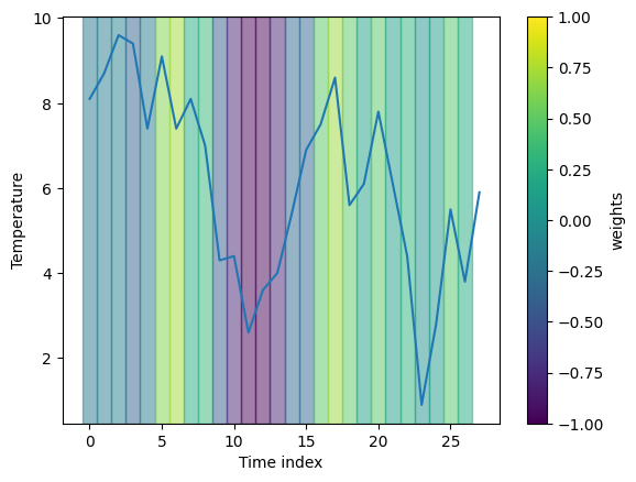
Now we can visualize the relevance scores on top of the displayed timeseries using the visualization tool in dianna.

heatmap_channel = normalize(exp[np.argmax(pred_onnx)])
segments = []
for i in range(len(heatmap_channel) - 1):
    segments.append({
        'index': i,
        'start': i - 0.5,
        'stop': i + 0.5,
        'weight': heatmap_channel[i]})
fig, _ = visualization.plot_timeseries(range(len(heatmap_channel)), data_instance[0],
                              segments, x_label="Time index", y_label="Temperature")

6 - Conclusions

The saliency scores are segment-wise relevances generated with LIME explainer.

The first example with a designed timeseries and an expert model demonstrates that LIME is able to identify the important segments for the classification in a simplified case.

The second example shows that LIME also runs on real timeseries data. The explanation is hard to interpret in this case, though. This could be due to an suboptimally trained model, unsuitable masking or segmentation strategy.